
A number of days in the past I wrote concerning the approximation
for cosine as a result of Indian astronomer Aryabhata (476–550) and gave this plot of the error.
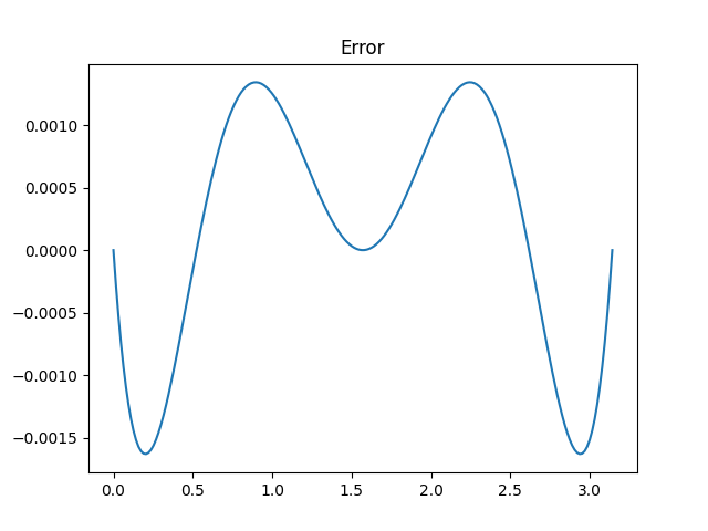 I mentioned that Aryabhata’s approximation is “not fairly optimum because the ripples within the error operate aren’t of equal peak.” This was an allusion to the equioscillation theorem.
Chebyshev proved that an optimum polynomial approximation has an error operate that has equally giant optimistic and destructive oscillations. Later this theorem was generalized to rational approximations via a sequence of outcomes by de la Vallée Poussin, Walsh, and Achieser. Right here’s the formal assertion of the concept from [1] within the context of real-valued rational approximations with numerators of diploma m and denominators of diploma n
Theorem 24.1. Equioscillation characterization of greatest approximants. An actual operate f in C[−1, 1] has a singular greatest approximation r*, and a operate r is the same as r* if and provided that f − r equioscillates between at the very least m + n + 2 − d extremes the place d is the defect of r.
When the concept says the error equioscillates, it means the error alternately takes on ± its most absolute worth.
The defect is non-zero when each numerator and denominator have lower than maximal diploma, which doesn’t concern is right here.
We wish to discover the optimum rational approximation for cosine over the interval [−π/2, π/2]. It doesn’t matter that the concept is acknowledged for steady features over [−1, 1] as a result of we may simply rescale cosine. We’re searching for approximations with (m, n) = (2, 2), i.e. ratios of quadratic polynomials, to see if we are able to enhance on the approximation on the prime of the submit.
The equioscillation theorem says our error ought to oscillate at the very least 6 instances, and so if we discover an approximation whose error oscillates as required by the concept, we all know we’ve discovered the optimum approximation.
I first tried discovering the optimum approximation utilizing Mathematica’s MiniMaxApproximation operate. However this operate tries to optimize relative error and I’m attempting to reduce absolute error. Minimizing relative error creates issues as a result of cosine evaluates to zero on the ends of interval ±π/2. I attempted a number of options and finally determined to take one other strategy.
As a result of the cosine operate is even, the optimum approximation is even. Which suggests the optimum approximation has the shape
(a + bx²) / (c + dx²)
and we are able to assume with out lack of generality that a = 1. I then wrote some Python code to reduce the error as a operate of the three remaining variables. The outcomes have been b = −4.00487004, c = 9.86024544, and d = 1.00198695, very near Aryabhata’s approximation that corresponds to b = −4, c = π², and d = 1.
Right here’s a plot of the error, the distinction between cosine and the rational approximation.
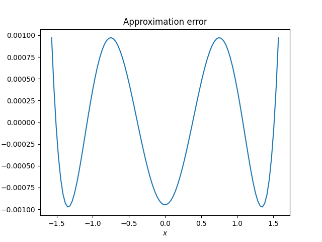
Absolutely the error takes on its most worth seven instances, alternating between optimistic and destructive values, and so we all know the approximation is perfect. Nonetheless sketchy my strategy to discovering the optimum approximation might have been, the plot exhibits that the result’s appropriate.
Aryabhata’s approximation had most error 0.00163176 and the optimum approximation has most error 0.00097466. We have been capable of shave about 1/3 off the utmost error, however at a price of utilizing coefficients that may be tougher to make use of by hand. This wouldn’t matter to a contemporary laptop, however it will matter an amazing deal to an historic astronomer.
Associated posts
[1] Approximation Theory and Approximation Practice by Lloyd N. Trefethen